


Excel Test for Job Interview — What You Really Need to Know
Looking to land your next job? Don’t be surprised if you’re asked to complete an Excel test during the interview. Whether it’s for an admin, finance, HR, or data role, employers often use Excel tasks to assess how comfortable you are with spreadsheets, formulas, and real-world problem solving.
In this blog, we’ll walk you through 5 essential Excel tasks that regularly show up in job interview tests — with clear examples and instructions. Plus, you can download a free PDF workbook with 10 more practice challenges at the end.
Let’s get started.
1. How to Use VLOOKUP in Excel
Employers want to see if you can pull data from another table using a matching key (like an Employee ID).
It’s a basic—but powerful—test of real-world Excel skills.
What to do:
- Formula format:
=VLOOKUP(lookup_value, table_array, col_index_num, FALSE) - Example: Find the department for employee ID 102 from a separate sheet.
- Use:
=VLOOKUP(102, Sheet2!A2:C100, 3, FALSE)
Example:
Step 1: Create Your Data
Sheet1: Main
| A (Employee ID) | B (Name) |
|---|---|
| 101 | Alice |
| 102 | John |
| 103 | David |
Sheet2: Employee_Info
| A (Employee ID) | B (Department) |
|---|---|
| 101 | Finance |
| 102 | HR |
| 103 | Marketing |
Make sure the Employee ID is in Column A in both sheets. That’s critical for VLOOKUP to work.
Step 2: Use This Formula in Sheet1
-
Go to Sheet1 (
Main) -
In cell C2, enter this formula:
=VLOOKUP(A2, Employee_Info!A:B, 2, FALSE) -
Press Enter
If done correctly, Excel will return “Finance” in C2.
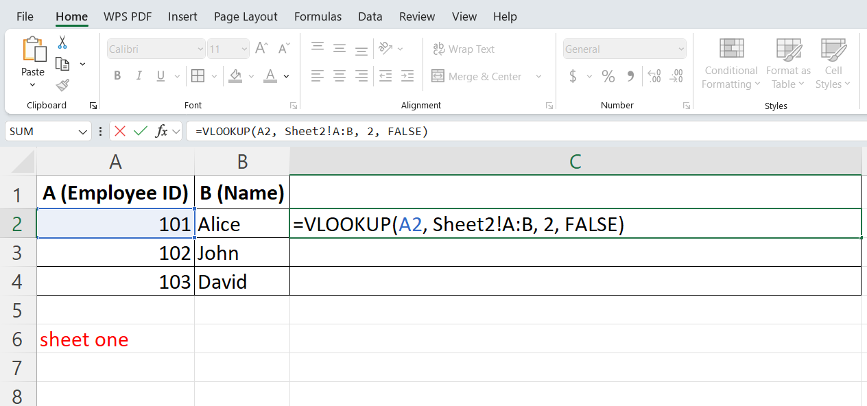
Entering VLOOKUP formula to the table
Step 3: Drag the Formula Down
-
Click on cell C2
-
Use the bottom-right corner handle to drag the formula down to C3 and C4
It will now return:
-
C3 → “HR”
-
C4 → “Marketing”
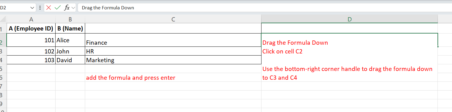
Final table
2. How to Use IF Formula for Pass/Fail Logic
Why it’s asked: Simple decision-making logic is used in everything from grading to project flags.
What to do:
- Formula:
=IF(A2>=50, "Pass", "Fail") - Application: Used for test scores, thresholds, or flagging records based on conditions.
Why It’s Asked in Interviews
Employers ask this to check if you can use basic logical conditions in spreadsheets.
This is crucial in real-world scenarios like:
-
Grading students
-
Flagging overdue tasks
-
Validating payment thresholds
-
Identifying project risks
Example -How to Use IF Formula for Pass/Fail Logic
If a score is 50 or above, return “Pass”
If it’s below 50, return “Fail”
Example Data Table
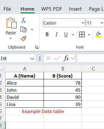
Example – data table
Entering Formula:
Go to column C (empty) and in cell C2, enter:=IF(B2>=50, "Pass", "Fail")
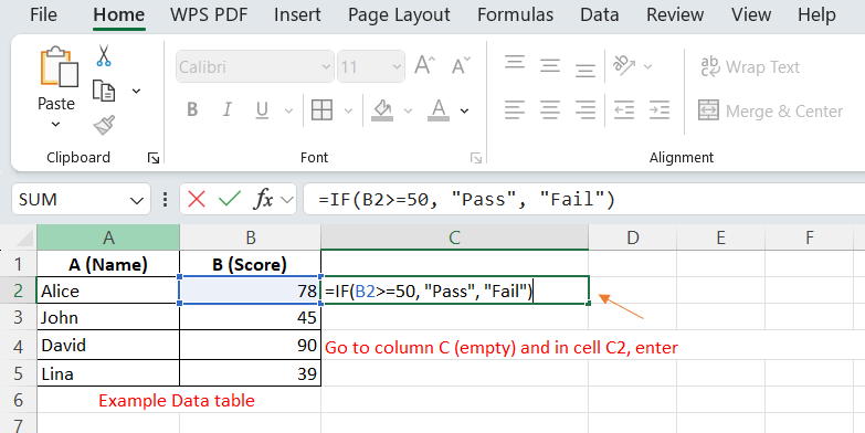
Adding IF Function
Explanation:
-
B2>=50→ checks if the score is 50 or more -
If TRUE → returns
"Pass" -
If FALSE → returns
"Fail"
Then drag the formula down to apply to the rest of the rows
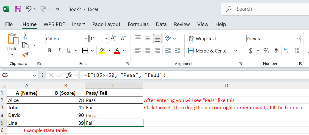
Final table – After using IF Function
3. How to Remove Duplicates in Excel
Why It’s Asked in Interviews
Removing duplicates is a common data cleaning task. Employers want to know if you can clean up customer lists, inventory sheets, or transaction logs — without errors or manual deletion.
It tests your ability to:
-
Work with structured data
-
Use Excel’s built-in cleanup tools
-
Preserve data integrity
Example -How to Remove Duplicates in Excel
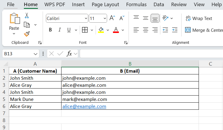
Data table
Your task is to remove duplicate customer records — not just the name, but exact matches of the full row (Name + Email).
Step-by-Step Instructions -How to Remove Duplicates in Excel
1. Select Your Data
Click and drag to highlight the entire range — including the column headers (e.g., A1:B6).
2. Go to Data Tab
Click the “Data” tab on the Excel ribbon.
3. Click “Remove Duplicates”
-
In the Data Tools group, click Remove Duplicates
-
A popup window will appear
4. Select Columns to Check
-
Ensure both “Customer Name” and “Email” are checked
-
This makes sure Excel compares the full row
-
Click OK
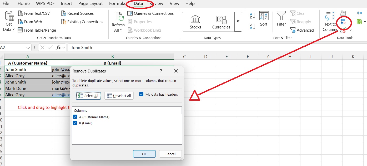
How to Remove Duplicates in Excel
5. Excel Removes Duplicates
A message will show how many duplicate values were removed and how many unique values remain.
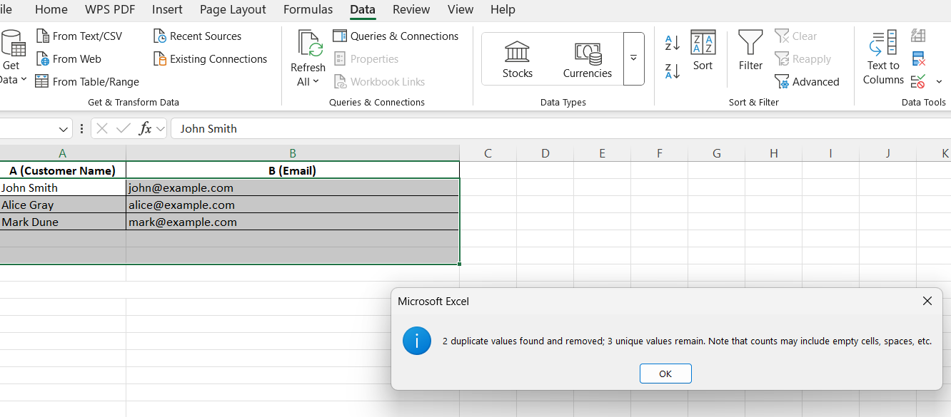
final result
Pro Tip:
-
Always make a copy of your data first, in case you want to restore anything later
-
You can also use “Advanced Filter” for more control over duplicates
4. How to Create a Pivot Table
Why It’s Asked in Interviews
PivotTables are one of Excel’s most powerful tools. They allow users to summarize, filter, and analyze large datasets without complex formulas. Recruiters want to know if you can turn raw data into meaningful summaries.
Example Scenario:
You are given a sales dataset with the following fields:
| Date | Sales Rep | Region | Amount |
|---|---|---|---|
| 01/01/2024 | Alice | North | 1500 |
| 01/02/2024 | John | South | 2000 |
| 01/02/2024 | Alice | North | 1200 |
| 01/03/2024 | Mark | West | 1700 |
You need to summarize total sales by Sales Rep.
Step-by-Step Instructions – How to Create a Pivot Table
1. Select Your Data
Click anywhere inside the data range (or select the full range A1:D5).
2. Insert Pivot Table
-
Go to Insert tab → Click on PivotTable → Choose: “Place PivotTable in New Worksheet” → Click OK
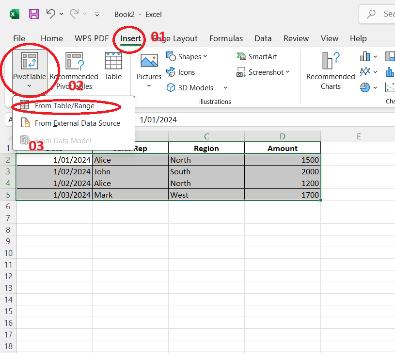
Inserting Pivot Table
3. Build Your PivotTable
Use the PivotTable Field Pane on the right:
-
Drag Sales Rep to Rows
-
Drag Amount to Values
-
(Optional) Drag Region to Filters
Excel will now summarize the total Amount for each Sales Rep.
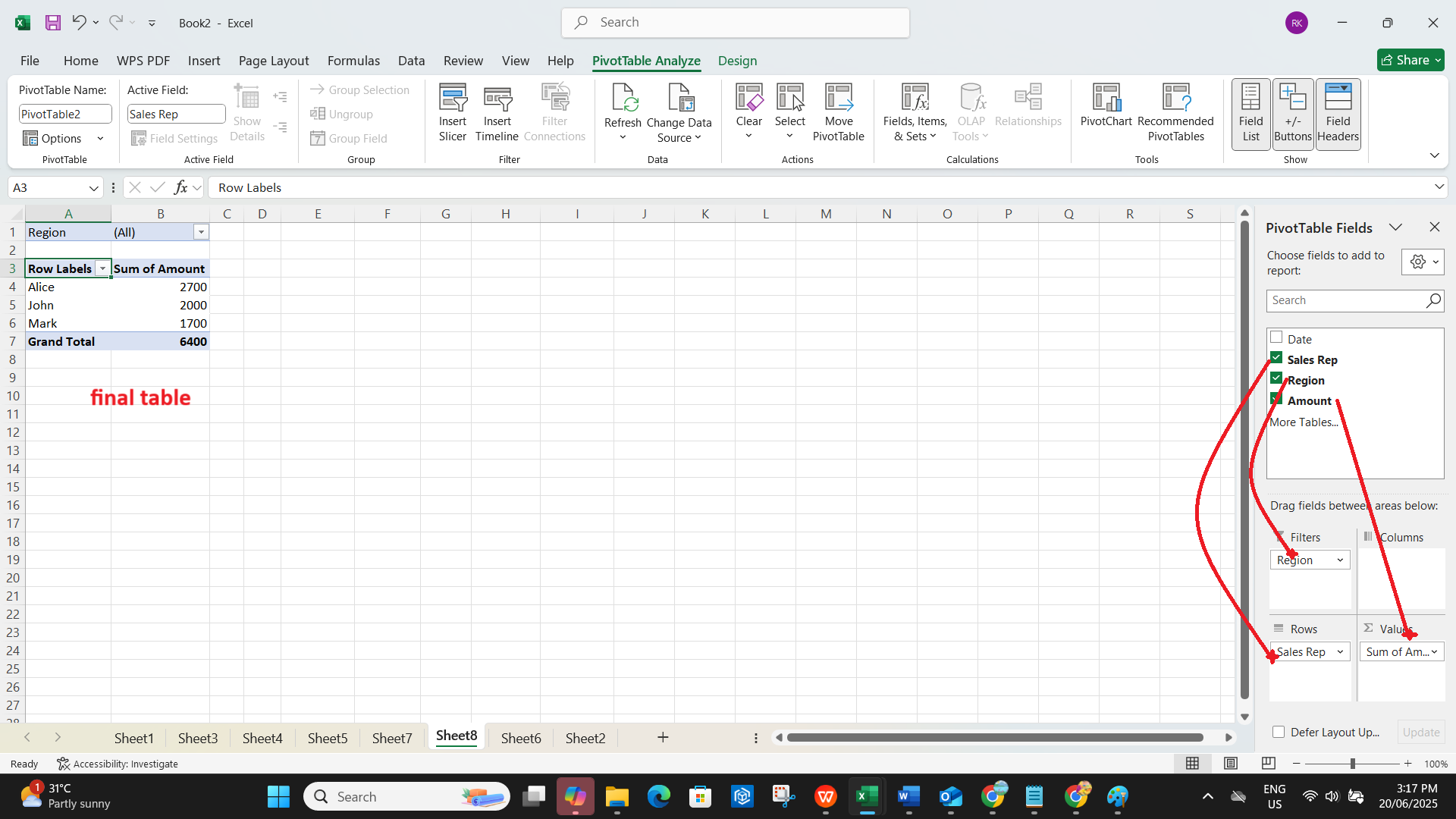
Building the PivotTable
Final Output:
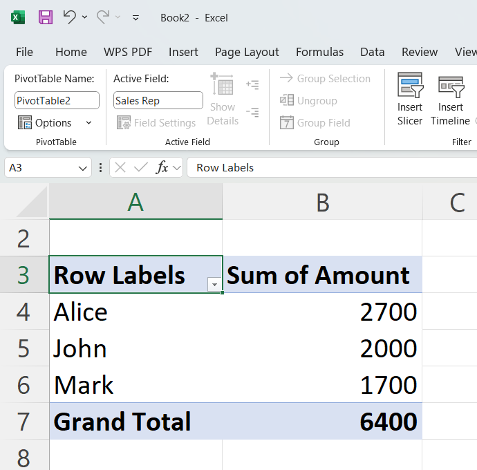
Final view of the pivot table
Pro Tips:
-
To change the summary type (e.g., Sum, Average, Count):
Click on the value in the Pivot > Value Field Settings -
You can group dates by Month, Quarter, Year:
Right-click a date > Group
5. How to Use Conditional Formatting in Excel
Why It’s Asked in Interviews
Conditional formatting lets users quickly identify values that meet certain conditions — for example, sales over target, overdue dates, or duplicate entries.
It shows your ability to visually interpret data, which is critical in business and reporting roles.
Example -How to Use Conditional Formatting in Excel
You have a list of sales amounts. You need to highlight values greater than 1000 for review.
| A (Sales Amount) | month |
| 850 | January |
| 1200 | February |
| 670 | March |
| 1900 | April |
| 1025 | May |
Step-by-Step Instructions -How to Use Conditional Formatting in Excel
Option 1: Use Built-In Rule
-
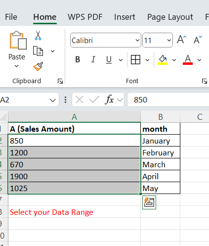
Select your data range
Example: Select A2:A6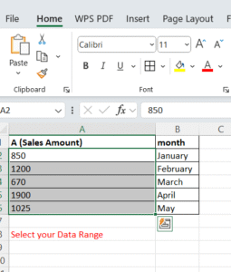
Selecting the Data range
-
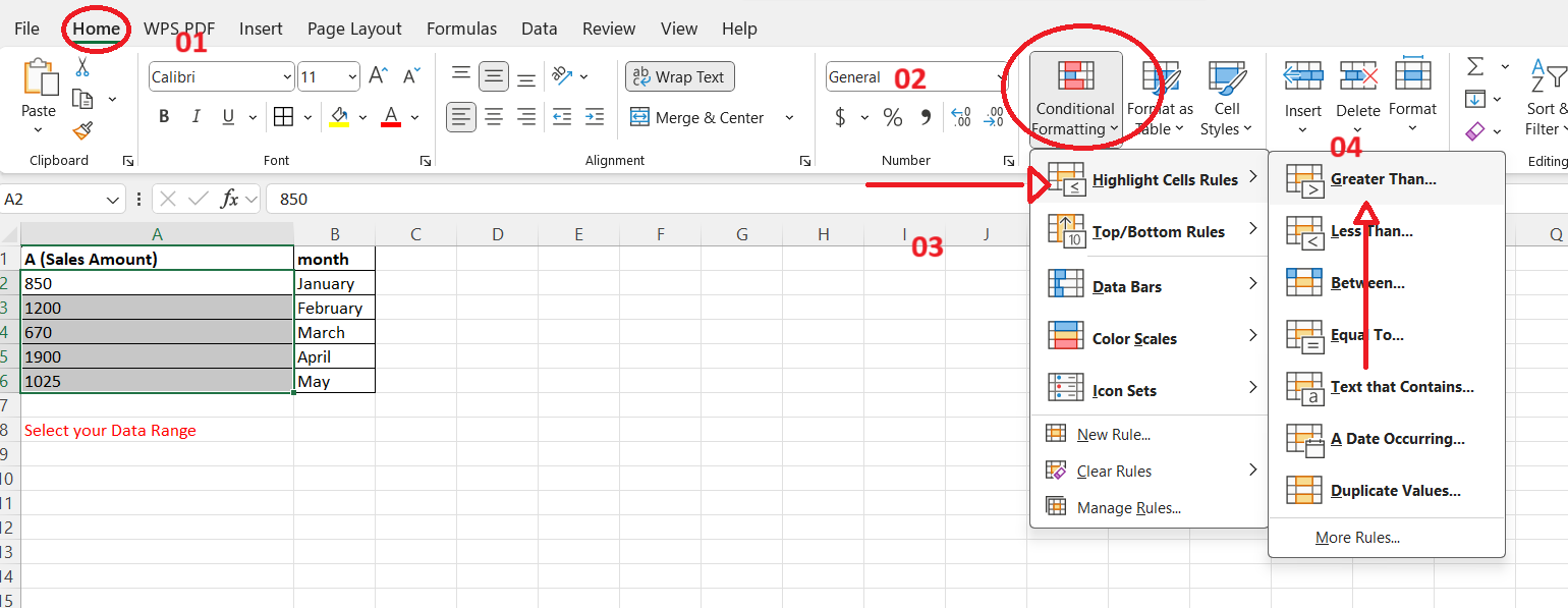
Go to the Home tab > Conditional Formatting
-
Choose:
Highlight Cells Rules > Greater Than…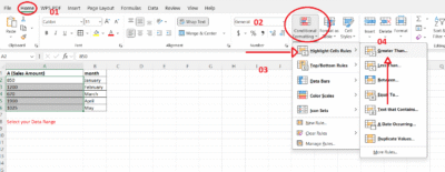
How to Use Conditional Formatting in Excel
-
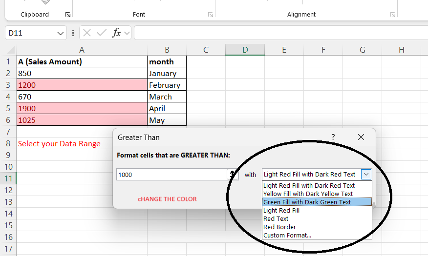
In the dialog box:
-
Enter
1000 -
Choose a formatting style (light red fill, yellow text, etc.)
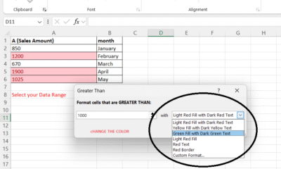
How to Use Conditional Formatting in Excel
-
-
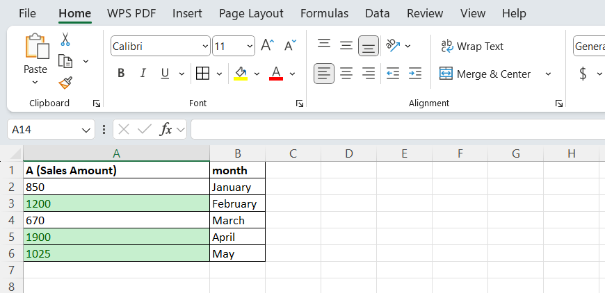
Click OK
All values above 1000 will be instantly highlighted.
final look – after adding conditional formatting to the data
Real Uses in Business:
-
Highlight overdue dates (
=TODAY()>DueDate) -
Flag underperforming sales reps (
=B2<5000) -
Shade alternate rows for readability (
=ISEVEN(ROW()))
Download the Full Excel Interview Test PDF (10 Extra Tasks)
Want more? We’ve created a free downloadable PDF with 10 additional realistic Excel tasks based on real job interview requirements. It includes cleaning tasks, formula work, chart creation, and more.
EXCEL PRACTICE TEST WITH ANSWER GUIDE pdf
Use it to:
- Practice under timed conditions
- Prepare for real Excel assessments
- Train new hires or assess candidates
Final Notes
These five Excel tasks are not only the most searched online — they’re also the most common in interviews. Mastering them shows that you’re comfortable with real-world spreadsheet responsibilities.
Don’t stop here. Use the downloadable PDF to expand your skills and simulate an actual Excel test.
Looking to sharpen your Excel skills even further? Get a full Microsoft Office license from UpkeyStore and start practicing with real tools today.
Related Links: